Varying Life Annuity Payments¶

Definition¶

A varying life annuity pays predetermined amounts $b_k\ge0$ at times $t_k$ conditional on survival. Its present value is $\displaystyle Y=\sum_k b_kv^{t_k}\indicator_{\{T_x>t_k\}}$ $k \sum b_{k} v^{t_{k}} 𝟙 1_{{T_{x} > t_{k}}}$ . For continuous rate $b(t)$ , replace the sum by $\int_0^{T_x}b(t)v^t\,\mathrm{d}t$ .

Interpretation¶

The indicator specifies eligibility for each payment. This representation handles increasing, decreasing and stepped benefits without treating them as separate probability models.

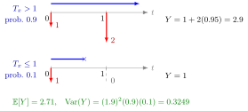
Two timelines for an annuity paying 1 now and 2 at time 1 if the life is alive: with survival the present value is 2.9, otherwise only the first payment of 1 is made.

The figure draws the example $Y=1+2v\indicator_{\{T_x>1\}}$ with $v=0.95$ and $p_x=0.9$ $0.9$ . The arrow lengths show the different scheduled amounts, and the survival indicator decides whether the second one is paid: $Y=2.9$ with probability $0.9$ and $Y=1$ with probability $0.1$ . Hence $\mathbb{E}[Y]=2.71$ $2.71$ , and since only the second payment is random, $\operatorname{Var}(Y)=(1.9)^2(0.9)(0.1)=0.3249$ $0.3249$ .

The whole life annuity-due is recovered by setting unit payments at integer dates. An indicator random variable switches each scheduled amount on only when the life survives to its date. Joint survival events explain the dependence between payments in the second-moment calculation.

Key Results¶

The actuarial present value (APV) is $\displaystyle \sum_k b_kv^{t_k}{}_{t_k}p_x$ , or $\int_0^\infty b(t)v^t{}_tp_x\,\mathrm{d}t$ for continuous payments.
Survival indicators at different dates are dependent. Their joint probability is ${}_{\max(t_j,t_k)}p_x$ .
Thus $\displaystyle \mathbb{E}[Y^2]=\sum_{j,k}b_jb_kv^{t_j+t_k}{}_{\max(t_j,t_k)}p_x$ $j, k \sum b_{j} b_{k} v^{t_{j} + t_{k}}_{m a x (t_{j}, t_{k})} p_{x}$ , when finite.
Do not calculate annuity variance by assuming independent annual payments.

Examples¶

The figure's example $Y=1+2v\indicator_{\{T_x>1\}}$ is worked out above: APV $2.71$ and variance $0.3249$ .

Increasing annuity-due. Payments $1,2,3$ at times $0,1,2$ , with $v=0.95$ $0.95$ , $p_x=0.9$ and ${}_2p_x=0.8$ $0.8$ . The APV is $1+2(0.95)(0.9)+3(0.95)^2(0.8)=1+1.71+2.166=4.876$ $4.876$ . The present value takes three values: $Y=1$ if $T_x\le1$ (probability $0.1$ ), $Y=2.9$ if $1<T_x\le2$ (probability $0.1$ ), and $Y=2.9+3(0.95)^2=5.6075$ if $T_x>2$ (probability $0.8$ ). So $\mathbb{E}[Y^2]=0.1+0.841+25.155245=26.096245$ and $\operatorname{Var}(Y)=26.096245-4.876^2\approx2.3209$ $2.3209$ . Treating the payments as independent would give only about $1.4978$ .

Prerequisites¶

Sources¶

Life Insurance · Lecture 6

Aliases: increasing life annuity, non-standard life annuity, varying annuity, increasing annuity, decreasing life annuity Keywords: dependent survival indicators, second moment of an annuity, stepped annuity payments, (Iä) x Symbols: infinity, integral, sum

Last updated: 17 October 2026 21:53